Download

This notebook can be downloaded as introduction-stripped.ipynb. See the button at the top right to download as markdown or pdf.

Introduction, Text Removed

This notebook has had all its explanatory text removed and has not been run. It is intended to be downloaded and run locally (or on the provided binder) while listening to the presenter’s explanation. In order to see the fully rendered of this notebook, go here

Questions

Throughout this notebook, there will be several questions that look like this. You are encouraged to stop and think about the question, to try and answer it yourself (perhaps looking at the hints that follow) before moving on and reading the answer below it.

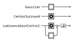
For the purposes of this notebook, we’ll use some very simple convolutional models that are inspired by the processing done in the lateral geniculate nucleus (LGN) of the visual system[1]. We’re going to build up in complexity, starting with the Gaussian model at the top and gradually adding features[2]. We’ll describe the components of these models in more detail as we get to them, but briefly:

• Gaussian: the model just convolves a Gaussian with an image, so that the model’s representation is simply a blurry version of the image.

• CenterSurround: the model convolves a difference-of-Gaussian filter with the image, so that model’s representation is bandpass, caring mainly about frequencies that are neither too high or too low.

• LuminanceGainControl: the model rectifies and normalizes the linear component of the response using a local measure of luminance, so that the response is invariant to local changes in luminance.

Plenoptic basics

import plenoptic as po
import torch
import pyrtools as pt
import matplotlib.pyplot as plt
# so that relative sizes of axes created by po.imshow and others look right
plt.rcParams['figure.dpi'] = 72
plt.rcParams['animation.html'] = 'html5'
# use single-threaded ffmpeg for animation writer
plt.rcParams['animation.writer'] = 'ffmpeg'
plt.rcParams['animation.ffmpeg_args'] = ['-threads', '1']

%matplotlib inline

DEVICE = torch.device('cuda' if torch.cuda.is_available() else 'cpu')
if DEVICE.type == 'cuda':
    print("Running on GPU!")
else:
    print("Running on CPU!")
# for reprodicibility
po.tools.set_seed(1)

img = po.data.einstein().to(DEVICE)
fig = po.imshow(img)

Set up the Guassian model. Models in plenoptic must:

• Inherit torch.nn.Module.

• Accept 4d tensors as input and return 3d or 4d tensors as output.

• Have forward and __init__ methods.

• Have all gradients removed.

# this is a convenience function for creating a simple Gaussian kernel
from plenoptic.simulate.canonical_computations.filters import circular_gaussian2d

# Simple Gaussian convolutional model
class Gaussian(torch.nn.Module):
    # in __init__, we create the object, initializing the convolutional weights and nonlinearity
    def __init__(self, kernel_size, std_dev=3):
        super().__init__()
        self.kernel_size = kernel_size
        self.conv = torch.nn.Conv2d(1, 1, kernel_size=kernel_size, padding=(0, 0), bias=False)
        self.conv.weight.data[0, 0] = circular_gaussian2d(kernel_size, float(std_dev))
        
    # the forward pass of the model defines how to get from an image to the representation
    def forward(self, x):
        x = po.tools.conv.same_padding(x, self.kernel_size, pad_mode='circular')
        return self.conv(x)

# we pick this particular number to match the models found in the Berardino paper
model = Gaussian((31, 31)).to(DEVICE)
rep = model(img)

print(img.shape)
print(rep.shape)

po.tools.remove_grad(model)
model.eval()

• The Gaussian model output is a blurred version of the input.

• This is because the model is preserving the low frequencies, discarding the high frequencies (i.e., it’s a lowpass filter).

• Thus, this model is completely insensitive to high frequencies – information there is invisible to the model.

fig = po.imshow(torch.cat([img, rep]), title=['Original image', 'Model output'])

Examining model invariances with metamers

• Initialize the Metamer object and synthesize a model metamer.

• View the synthesis process.

metamer = po.synthesize.Metamer(img, model)

matched_im = metamer.synthesize(store_progress=True, max_iter=20)
# if we call synthesize again, we resume where we left off
matched_im = metamer.synthesize(store_progress=True, max_iter=150)

po.synthesize.metamer.plot_loss(metamer);

Important

This next cell will take a while to run — making animations in matplotlib is a bit of a slow process.

po.synthesize.metamer.animate(metamer, included_plots=['display_metamer', 'plot_loss'], figsize=(12, 5))

fig = po.imshow([img, rep, metamer.metamer, model(metamer.metamer)], 
                col_wrap=2, vrange='auto1',
                title=['Original image', 'Model representation\nof original image',
                       'Synthesized metamer', 'Model representation\nof synthesized metamer']);

Question

Why does the model metamer look “staticky”?

Hint

Model metamers help us examine the model’s nullspace, its invariances. A Gaussian is a lowpass filter, so what information is it insensitive to?

• Synthesize more model metamers, from different starting points.

curie = po.data.curie().to(DEVICE)
# pyrtools, imported as pt, has a convenience function for generating samples of white noise, but then we still 
# need to do some annoying things to get it ready for plenoptic
pink = torch.from_numpy(pt.synthetic_images.pink_noise((256, 256))).unsqueeze(0).unsqueeze(0)
pink = po.tools.rescale(pink).to(torch.float32).to(DEVICE)
po.imshow([curie, pink]);

metamer_curie = po.synthesize.Metamer(img, model, initial_image=curie)
metamer_pink = po.synthesize.Metamer(img, model, initial_image=pink)

# we increase the length of time we run synthesis and decrease the
# stop_criterion, which determines when we think loss has converged
# for stopping synthesis early.
metamer_curie.synthesize(max_iter=500,  stop_criterion=1e-7)
metamer_pink.synthesize(max_iter=500,  stop_criterion=1e-7)

po.synthesize.metamer.plot_loss(metamer_curie)
po.synthesize.metamer.plot_loss(metamer_pink);

In the following plot:

• the first row shows our target Einstein image and its model representation, as we saw before.

• the new three rows show our model metamers resulting from three different starting points.

• in each, the first column shows the starting point of our metamer synthesis, the middle shows the resulting model metamer, and the third shows the model representation.

We can see that the model representation is the same for all four images, but the images themselves look very different. Because the model is completely invariant to high frequencies, the high frequencies present in the initial image are not affected by the synthesis procedure and thus are still present in the model metamer.

fig = po.imshow([torch.ones_like(img), img, rep,
                 metamer.saved_metamer[0], metamer.metamer, model(metamer.metamer),
                 pink, metamer_pink.metamer, model(metamer_pink.metamer),
                 curie, metamer_curie.metamer, model(metamer_curie.metamer)],
                col_wrap=3, vrange='auto1',
                title=['', 'Original image', 'Model representation\nof original image']+
                      3*['Initial image', 'Synthesized metamer', 'Model representation\nof synthesized metamer']);

Examining model sensitivies to eigendistortions

• While metamers allow us to examine model invariances, eigendistortions allow us to also examine model sensitivities.

• Eigendistortions are distortions that the model thinks are the most and least noticeable.

• They can be visualized on their own or on top of the reference image.

eig = po.synthesize.Eigendistortion(img, model)
eig.synthesize();

po.imshow(eig.eigendistortions, title=['Maximum eigendistortion', 
                                       'Minimum eigendistortion']);

po.imshow(img + 3*eig.eigendistortions, title=['Maximum eigendistortion', 
                                               'Minimum eigendistortion']);

A more complex model

• The CenterSurround model has bandpass sensitivity, as opposed to the Gaussian’s lowpass.

• Thus, it is still insensitive to the highest frequencies, but it is less sensitive to the low frequencies the Gaussian prefers, with its peak sensitivity lying in a middling range.

# These values come from Berardino et al., 2017.
center_surround = po.simulate.CenterSurround((31, 31), center_std=1.962, surround_std=4.235,
                                             pad_mode='circular').to(DEVICE)
po.tools.remove_grad(center_surround)
center_surround.eval()
center_surround(img).shape

po.imshow([img, center_surround(img)]);

• We can synthesize all three model metamers at once by taking advantage of multi-batch processing.

white_noise =  po.tools.rescale(torch.rand_like(img), a=0, b=1).to(DEVICE)
init_img = torch.cat([white_noise, pink, curie], dim=0)
# metamer does a 1-to-1 matching between initial and target images,
# so we need to repeat the target image on the batch dimension
cs_metamer = po.synthesize.Metamer(img.repeat(3, 1, 1, 1), center_surround, initial_image=init_img)
cs_metamer.synthesize(1000, stop_criterion=1e-7)

Show code cell source Hide code cell source

# this requires a little reorganization of the tensors:
to_plot = [torch.cat([torch.ones_like(img), img, center_surround(img)])]
for i, j in zip(init_img, cs_metamer.metamer):
    to_plot.append(torch.stack([i, j, center_surround(j)]))
to_plot = torch.cat(to_plot)
fig = po.imshow(to_plot, col_wrap=3, 
                title=['', 'Original image', 'Model representation\nof original image']+
                       3*['Initial image', 'Synthesized metamer', 'Model representation\nof synthesized metamer']);
# change the color scale of the images so that the first two columns go from 0 to 1 
# and the last one is consistent
for ax in fig.axes:
    if 'representation' in ax.get_title():
        clim = (to_plot[2::3].min(), to_plot[2::3].max())
    else:
        clim = (0, 1)
    ax.images[0].set_clim(*clim)
    title = ax.get_title().split('\n')
    title[-2] = f" range: [{clim[0]:.01e}, {clim[1]:.01e}]" 
    ax.set_title('\n'.join(title))

Question

How do these model metamers differ from the Gaussian ones? How does that relate to what we know about the model’s sensitivities and invariances?

• By examining the eigendistortions, we can see more clearly that the model’s preferred frequency has shifted higher, while the minimal eigendistortion still looks fairly similar.

cs_eig = po.synthesize.Eigendistortion(img, center_surround)
cs_eig.synthesize();
po.imshow(cs_eig.eigendistortions, title=['Maximum eigendistortion', 
                                          'Minimum eigendistortion']);

Adding some nonlinear features to the mix

• The LuminanceGainControl model adds a nonlinearity, gain control. This makes the model harder to reason than the first two models.

• This is a computation that we think is present throughout much of the early visual system.

lg = po.simulate.LuminanceGainControl((31, 31), pad_mode="circular").to(DEVICE)
params_dict = {'luminance_scalar': 14.95, 'luminance.std': 4.235, 
               'center_surround.center_std': 1.962, 'center_surround.surround_std': 4.235,
               'center_surround.amplitude_ratio': 1.25}
lg.load_state_dict({k: torch.as_tensor([v]) for k, v in params_dict.items()})
po.tools.remove_grad(lg)
lg.eval()

po.imshow([lg(img), lg(2*img)], vrange='auto1');

lg_metamer = po.synthesize.Metamer(img.repeat(3, 1, 1, 1), lg, initial_image=init_img)
opt = torch.optim.Adam([lg_metamer.metamer], .007, amsgrad=True)
lg_metamer.synthesize(3500, stop_criterion=1e-11, optimizer=opt)

• The model metamers here look fairly similar to those of the CenterSurround model, though you can see these are more “gray”, because this model is even less sensitive to the local luminance than the previous model.

Show code cell source Hide code cell source

# this requires a little reorganization of the tensors:
to_plot = [torch.cat([torch.ones_like(img), img, center_surround(img)])]
for i, j in zip(init_img, lg_metamer.metamer):
    to_plot.append(torch.stack([i, j, center_surround(j)]))
to_plot = torch.cat(to_plot)
fig = po.imshow(to_plot, col_wrap=3, 
                title=['', 'Original image', 'Model representation\nof original image']+
                       3*['Initial image', 'Synthesized metamer', 'Model representation\nof synthesized metamer']);
# change the color scale of the images so that the first two columns go from 0 to 1 
# and the last one is consistent
for ax in fig.axes:
    if 'representation' in ax.get_title():
        clim = (to_plot[2::3].min(), to_plot[2::3].max())
    else:
        clim = (0, 1)
    ax.images[0].set_clim(*clim)
    title = ax.get_title().split('\n')
    title[-2] = f" range: [{clim[0]:.01e}, {clim[1]:.01e}]" 
    ax.set_title('\n'.join(title))

lg_eig = po.synthesize.Eigendistortion(img, lg)
lg_eig.synthesize();
po.imshow(lg_eig.eigendistortions, title=['Maximum eigendistortion', 
                                          'Minimum eigendistortion']);

Question

How do these eigendistortions compare to that of the CenterSurround model? Why do they, especially the maximum eigendistortion, look more distinct from those of the CenterSurround model than the metamers do?

Hint

The maximum eigendistortion emphasizes what the model is most sensitive to (whereas metamers focus on model invariances), so what about the LinearGainControl model’s nonlinearities would cause this change?

• Gain control makes this model adaptive, and thus the location of the eigendistortion matters, which was not true of our previous, linear models.

lg_curie_eig = po.synthesize.Eigendistortion(curie, lg)
lg_curie_eig.synthesize();
po.imshow(lg_curie_eig.eigendistortions, title=['LG Maximum eigendistortion\n (on Curie)', 
                                                'LG Minimum eigendistortion\n (on Curie)']);
cs_curie_eig = po.synthesize.Eigendistortion(curie, center_surround)
cs_curie_eig.synthesize();
po.imshow(cs_curie_eig.eigendistortions, title=['CenterSurround Maximum \neigendistortion (on Curie)', 
                                                'CenterSurround Minimum \neigendistortion (on Curie)']);
po.imshow(cs_eig.eigendistortions, title=['CenterSurround Maximum \neigendistortion (on Einstein)', 
                                          'CenterSurround Minimum \neigendistortion (on Einstein)']);

# the [:1] is a trick to get only the first element while still being a 4d
# tensor
po.imshow([img+3*lg_eig.eigendistortions[:1],
           curie+3*lg_curie_eig.eigendistortions[:1]]);

po.imshow(img+3*lg_eig.eigendistortions[:1].roll(128, -1))
print(f"Max LG eigendistortion: {po.tools.l2_norm(lg(img), lg(img+lg_eig.eigendistortions[:1]))}")
print(f"Shifted max LG eigendistortion: {po.tools.l2_norm(lg(img), lg(img+lg_eig.eigendistortions[:1].roll(128, -1)))}")

print(f"Max CenterSurround eigendistortion: {po.tools.l2_norm(center_surround(img), center_surround(img+cs_eig.eigendistortions[:1]))}")
print(f"Shifted max CenterSurround eigendistortion: {po.tools.l2_norm(center_surround(img), center_surround(img+cs_eig.eigendistortions[:1].roll(128, -1)))}")

Conclusion

In this notebook, we saw the basics of using plenoptic to investigate the sensitivities and invariances of some simple convolutional models, and reasoned through how the model metamers and eigendistortions we saw enable us to understand how these models process images.

plenoptic includes a variety of models and model components in the plenoptic.simulate module, and you can (and should!) use the synthesis methods with your own models. Our documentation also has examples showing how to use models from torchvision (which contains a variety of pretrained neural network models) with plenoptic. In order to use your own models with plenoptic, check the documentation for the specific requirements, and use the validate_model function to check compatibility. If you have issues or want feedback, we’re happy to help — just post on the Github discussions page!

---

[1]

Most of these models were originally published in Berardino, A., Laparra, V., J Ball’e, & Simoncelli, E. P. (2017). Eigen-distortions of hierarchical representations. In Adv. Neural Information Processing Systems (NIPS*17), from which the figure is modified.

[2]

Note that the Berardino et. al, 2017 paper includes more models than described here. We’re not examining all of them for time’s sake, but you can check out the rest of the models described in the Berardino paper, they’re all included in plenoptic under the plenoptic.simulate.FrontEnd module!